Multivariable Calculus (Calc III) - Complete Semester Course - Optimization over bounded regions, Multivariable Calculus

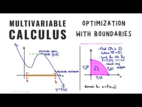
Finding the absolute maximum and absolute minimum values of z=f(x,y) over closed bounded domains in the xy-plane. (Multivariable Calculus Unit 3 Lecture 16) Step 1: Critical Points within Domain The first step in optimization involves identifying critical points within the subset of the domain (denoted as Ω). These are points where the gradient of the function is zero. (This process is what we did in the previous lecture, but in this situation, we may be looking at a restricted subset Ω of the function's entire domain.) These critical points are potential candidates for absolute extrema. Step 2: Boundary Curve(s) Parameterization We then parametrize any boundary curves of Ω. This step involves creating parametric equations for the boundaries of Ω and then evaluating the function 𝑓 along these curves. Optimization Along Boundaries Once the boundary curves are parameterized, we optimize the compositions 𝑓(𝑟⃗ 1(𝑡)), 𝑓(𝑟⃗ 2(𝑡)), etc., where 𝑟⃗ 𝑖(𝑡) are the parametric representations of the boundary curves. We differentiate these compositions with respect to 𝑡 and find critical points along each boundary curve by looking for places where 𝑑/𝑑𝑡 (𝑓∘𝑟⃗ (𝑡))=0. We only need to collect the points which are relevant to our domain. Step 3: Endpoints Evaluation In addition to critical points and boundary optimizations, we also consider any endpoints of the boundary curves. These endpoints might be locations where the function attains absolute extrema. Summary: Steps for Finding Absolute Extrema 1. Identify Critical Points: Find points within Ω where the gradient of the function is zero. 2. Parameterize Boundary Curves: Develop parametric equations for each boundary curve in 𝜔. 3. Optimize Function Along Boundaries: Differentiate the function compositions along the boundary curves to find critical points. 4. Evaluate Endpoints: Check any endpoints of the boundary curves as potential locations for extrema. Our first example is optimization over a closed disk (solid circle): Consider the function 𝑓(𝑥,𝑦)=𝑦𝑒^𝑥 over the domain Ω defined by 𝑥2+𝑦2≤1. This domain is a closed unit disk. 1. Gradient Computation: The gradient of 𝑓 is never zero, thus there are no traditional critical points within Ω. 2. Boundary Curve Parameterization: The boundary curve is the unit circle, parameterized as 𝑟⃗ (𝑡)=(cos(𝑡),sin(𝑡)) for 𝑡 from 0 to 2𝜋. 3. Function Composition Optimization: We optimize 𝑓(𝑟⃗ (𝑡))=sin(𝑡)𝑒^cos(𝑡), finding critical points along the boundary. 4. Endpoints Evaluation: The unit circle parametrization has no endpoints, so this step is skipped in this example. 5. Testing Points: We test the function at critical points along the boundary to find the absolute maxima and minima. Example: Optimization Subject to Constraints We optimize 𝑓(𝑥,𝑦) = 𝑥^2+𝑦^2 subject to the constraints 𝑥^2+4𝑦^2 ≤ 1 and 𝑦 ≥ 0. The domain is the upper half of an ellipse. 1. Critical Points Identification: The only critical point within the domain is at the origin. 2. Boundary Curves Parameterization: We parameterize the elliptical boundary and the line segment on the 𝑥-axis. 3. Optimize Along Boundaries: We find critical points along these boundary curves. 4. Evaluate Endpoints: Check endpoints of the boundary curves. 5. Test All Points: Evaluate the function at all these points to find the absolute maximum and minimum values. #calculus #multivariablecalculus #mathematics #optimization #partialderivatives #criticalpoint #iitjammathematics #calculus3