A full course in econometrics - undergraduate level - part 1 - The qualitative difference between stationary and non-stationary AR(1)

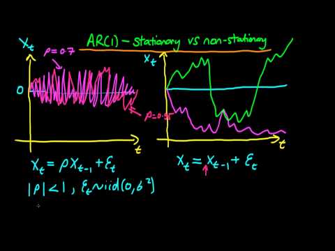
This video explains the qualitative difference between stationary and non-stationary AR(1) processes, and provides a simulation at the end in Matlab/Octave to demonstrate the difference. clear; close all; clc; n=10000; % Setting the number of time periods equal to 10000. b=1; rho=1; %This is the coefficient on the lagged part of x x=zeros(n,1); % Initialise the vector x x(1)=0; for i = 2:n x(i)=rho*x(i-1)+b*randn(); end zoom=1.0; FigHandle = figure('Position', [750, 300, 1049*zoom, 895*zoom]); plot(x, 'LineWidth', 1.4) ylabel('X(t)') xlabel('t') I also include the same in R (Courtesy of Jesse Maurais): z = rnorm(1000) gen = function(rho) { x = numeric(length(z)) x[1] = z[1] for (i in 2:length(z)) { x[i] = rho*x[i-1] + z[i] } x } display = function(rho) { x = gen(rho) plot(x, main=as.character(rho)) lines(x) } for (it in 1:100) { display(it/100) Sys.sleep(0.5) } Check out https://ben-lambert.com/econometrics-course-problem-sets-and-data/ for course materials, and information regarding updates on each of the courses. Quite excitingly (for me at least), I am about to publish a whole series of new videos on Bayesian statistics on youtube. See here for information: https://ben-lambert.com/bayesian/ Accompanying this series, there will be a book: https://www.amazon.co.uk/gp/product/1473916364/ref=pe_3140701_247401851_em_1p_0_ti